Disclaimer: If you haven’t read/watched day 5, I recommend you do that before reading this article.

For those of you who prefer to watch a video I made on my channel regarding my journey:

While using gradient descent for minimizing our cost function can be nice it takes many iterations and also requires us to select a good “learning rate” ($\alpha$) which can be quite tricky. That is when the normal equation comes in!

The Normal Equation

The normal equation is a non-iterative algorithm that will minimize our cost function ($J_\theta$) by explicitly taking its partial derivatives with respect to the $\theta_j$’s, and setting them to zero. This allows us to find the optimum theta without iterations.

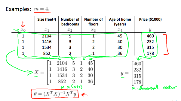
The normal equation formula is the following: $\theta = (X^TX)^{-1}X^Ty$

Example of Using The Normal Equation

Let’s say we want to predict the price of a house based on its size ($x_1$), number of bedrooms ($x_2$), number of floors ($x_3$) and the age of the home ($x_4$). In that case, given 4 training examples $X$ and $y$ are constructed in the following way:

What Happens If $X^TX$ Is Noninvertible

There can be many causes for this problem, but, the common causes are:

• Redundant features - two features are very closely related -> they are probably linearly dependent.

• Too many features ($m ≤ n$) - in this case, we might need to delete some features.

When To Use The Gradient Descent Over The Normal Equation?

If you think like me, you might be thinking to yourself that there is no reason not to use the normal equation, it just sounds better. Well, that is not always the case.

Since computing the inversion of a matrix has a time complexity of $O(n^3)$, if we have a large number of features, the normal equation will be slow (notice that $X^TX$ dimensions are (n+1)x(n+1)). In practice, when n exceeds 10000 it might be a good time to use gradient descent.

Note: If you have noticed something I haven’t talked about in this article is “feature scaling”. Well, that’s because you don’t need to, that is another one of the advantages of the normal equation method.